Purpose of the tool
Procedure
Settings
Interpretation guide
Forms of representation
Requirements
Tools
Examples
Terms
Formulas
Normality test
-
Purpose of the tool
The normality test is used to determine whether the available data can be adequately described by a normal distribution. Many statistical methods, such as process capability analysis using Cp and Cpk, require normally distributed data. The test provides an indication of whether this requirement is met and whether further analyses can be conducted on this basis. To do this, we examine the p-value: If the p-value is greater than 0.05, the data are treated as approximately normally distributed.
However, a p-value > 0.05 does not mean that the data are considered “proven to be normally distributed.” It merely indicates that there is no statistical evidence of a deviation from the normal distribution.
-
Example: Tomato Sauce
Viscosity values are regularly recorded during the production of tomato sauce. Before further analyses can be performed, it must be determined whether the measured values are approximately normally distributed.
The p-value is 0.111. Since this is greater than 0.05, there is no evidence of a deviation from the normal distribution. The data can therefore be treated as approximately normally distributed.

Probability Plot
The probability plot is a graphical tool used to check whether the data roughly resembles a normal distribution.
To do this, the measured values are sorted by magnitude and compared with the values that would be expected in a perfect normal distribution.
- If the points lie close to the drawn line, the data behaves as a normal distribution would.
- If the points lie far from the line or form a curve, this indicates that the data is not normally distributed.
- Typical patterns such as S-shapes, strong curves, or outliers indicate that the data deviates significantly from a normal distribution.
You can think of the line as a “template”:
The better the points fit on it, the more likely the data is normally distributed.
Anderson
In addition to the plot (probability plot), there is also a statistical test: the Anderson-Darling test.
This test uses calculations to check whether the data fits a normal distribution.
The test returns a p-value:
- p-value greater than 0.05:
There is no evidence that the data deviates from a normal distribution.
→ The data can be considered approximately normally distributed. - p-value less than or equal to 0.05:
The test finds significant deviations from the normal distribution.
→ The data is considered non-normally distributed
Why is the Anderson-Darling test often used?
It is particularly sensitive to deviations at the beginning and end of the distribution (i.e., where outliers are located). As a result, it detects anomalies more frequently than other tests and provides more reliable results in practice.
-
Procedure
(How was this graphic created?)
Preliminary Work
Select a continuous measurement parameter and collect measurement data (e.g., viscosity).
 Use in AlphadiTab
- In the Measure phase, select the Test for Normal Distribution tool.
- Select the “Viscosity” column.
- Generate a chart using the “Create New” button.
Interpretation
Use the p-value to determine whether the data can be considered normally distributed:
- p > 0.05 → The null hypothesis is not rejected. There is no evidence of a deviation from the normal distribution. The data can be treated as approximately normally distributed.
- p ≤ 0.05 → The null hypothesis is rejected. The data are considered non-normally distributed.
-
Requirements
Appropriate measuring equipment
Data must be collected using reliable measuring equipment that is suitable for the characteristic in order to ensure accurate results.
Why is this important?
Unsuitable measuring equipment can create the impression that the data is not normally distributed, even though the issue lies solely with the equipment.
-
Tools
(When are other options more suitable?)
For nominal or ordinal data, a test for normal distribution is not appropriate, as these data types cannot, by definition, be normally distributed. A normal distribution requires continuous measurement values.
Although discrete data (e.g., count data) may in some cases approximate a normal distribution—particularly with larger samples—you should always verify whether this assumption is appropriate for the specific application.
If you need to test multiple distributions simultaneously, the “Distribution Test” tool is more suitable. It offers a selection of continuous distributions that can be automatically compared with one another.
Production / Quality Assurance
Net weight of tomato sauce
In this example, the fill volume of the tomato sauce was examined. Each container is supposed to hold 500 ml. Before the quality of the filling process can be assessed, it is determined whether the measured fill volumes follow a typical normal distribution.
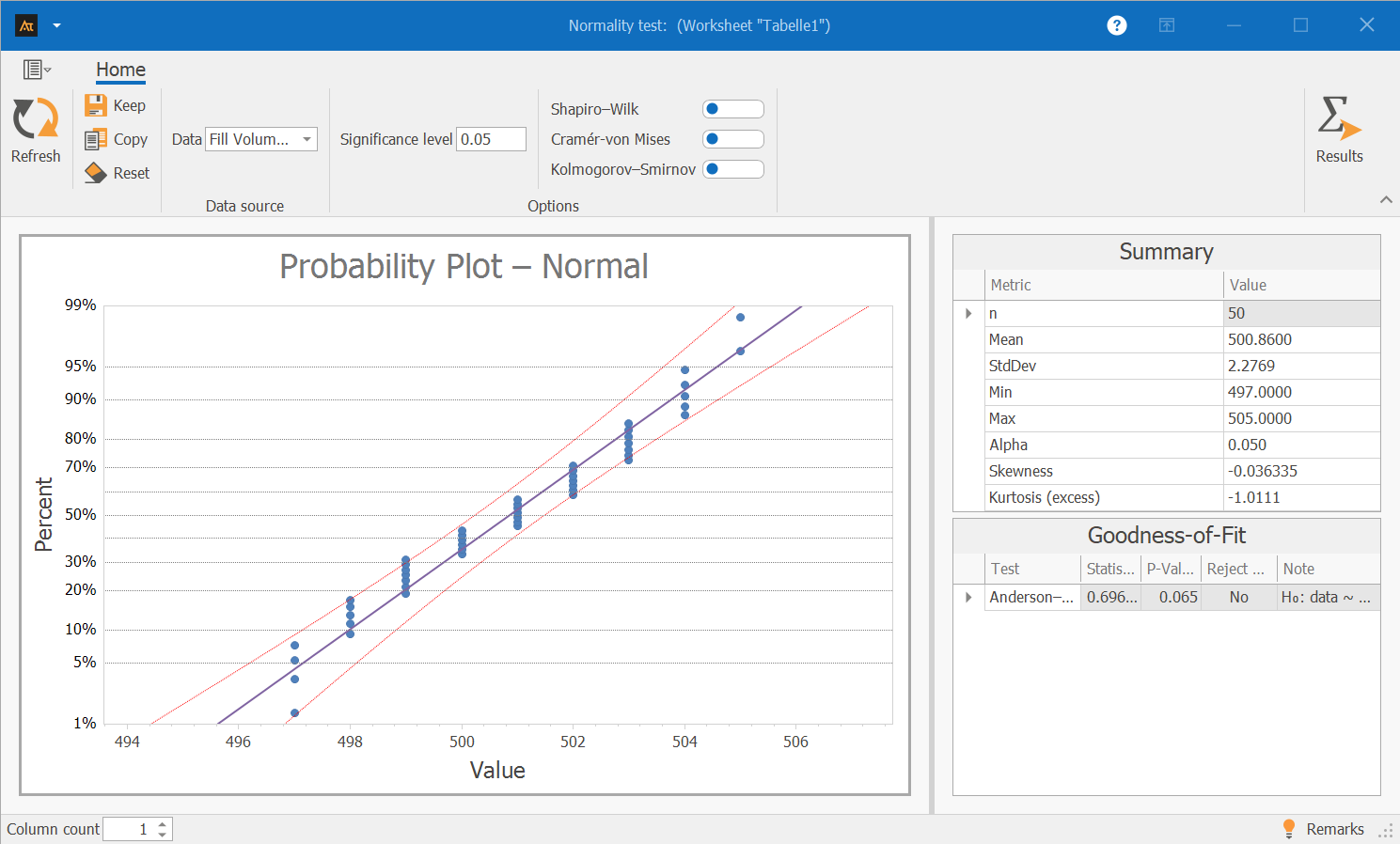
Interpretation:
In the probability plot, the data points lie predominantly on the plotted straight line. No major deviations or systematic patterns are apparent.
The Anderson-Darling test yields a p-value of 0.065. Since the p-value is greater than 0.05, there is no evidence of a significant deviation from the normal distribution. The data can therefore be treated as approximately normally distributed.
The visible frequency clusters may result from the resolution of the measuring instrument or from rounded values. However, they do not represent an anomaly with respect to the distribution. Overall, the data follow the normal distribution sufficiently well that they can be treated as approximately normally distributed for further analysis.
Goods Receiving/Logistics
Order processing time
In the receiving department, every order goes through an inspection process during which delivery notes are checked and items are entered into the system. While some processes are handled quickly, others get bogged down: a missing barcode, an incomplete delivery note, or a brief inquiry can cause individual orders to be held up longer. This results in highly variable processing times, which are clearly reflected in the measurement data. The goal is to determine whether the data is approximately normally distributed.
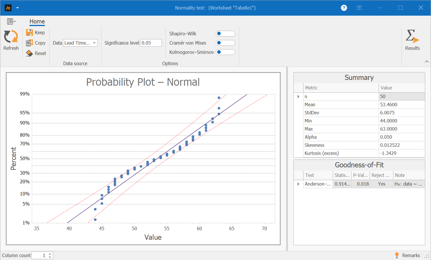
Interpretation:
In the probability plot, the data points deviate significantly from the line. Especially in the lower and middle ranges, it is clear that the data do not follow the typical pattern of a normal distribution.
The Anderson-Darling test confirms this visual assessment: The p-value is 0.018, which is below 0.05. The null hypothesis of a normal distribution is therefore rejected: The data are not normally distributed.
IT Support
Response Time for Inquiries
The IT service desk receives many different types of requests every day. Some tickets can be resolved immediately because the solution is obvious or a brief note is sufficient. Other inquiries first require follow-up questions, a system search, or the reproduction of an error. While simple cases are processed quickly, the response time for more complex tickets is significantly delayed. This results in widely varying response times—even though the goal is to keep the response time under 35 minutes. We need to check whether the data is approximately normally distributed.
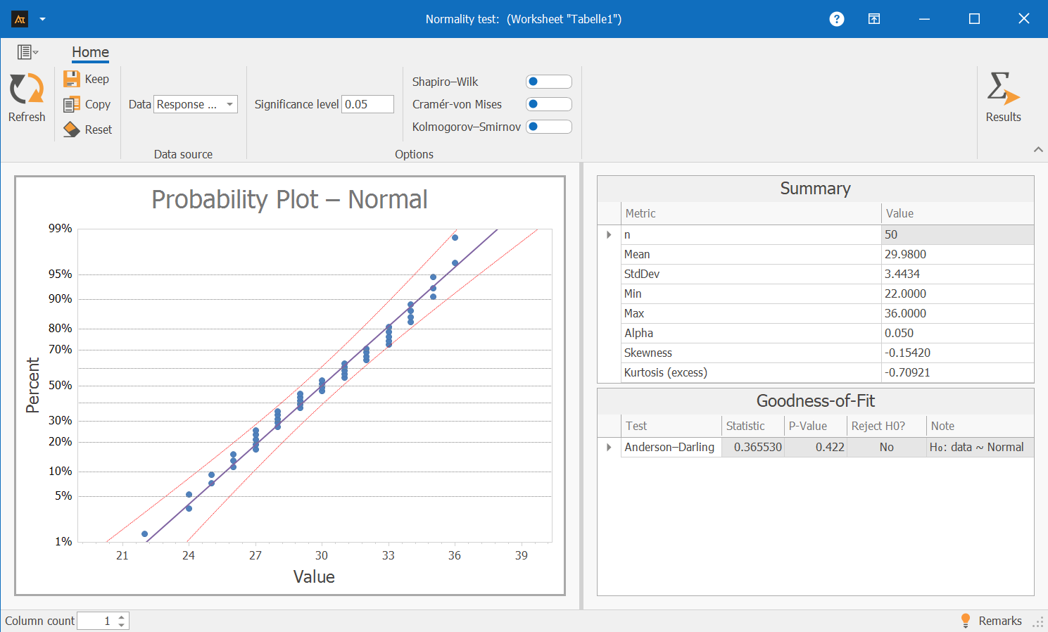
Interpretation:
In the probability plot, the data points are predominantly very close to the red line. No systematic deviations are apparent, and the pattern of points follows the expected distribution of a normal distribution.
The Anderson-Darling test confirms this impression: The p-value is 0.422, which is well above 0.05. There is therefore no evidence of a significant deviation from the normal distribution.
The data can be treated as approximately normally distributed.
Development
Service life of ball bearings
Ball bearings for a new machine type are tested under continuous operation. Each bearing remains on the test bench until it is no longer functional. This process generates service life data that is used to assess component reliability. The aim is to determine whether the data is approximately normally distributed.
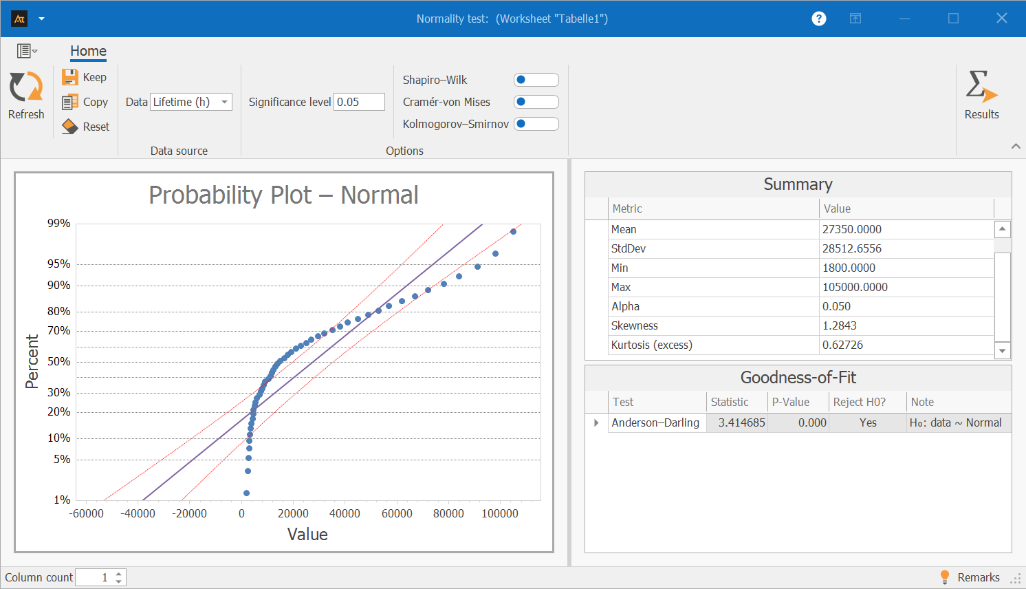
In the probability plot, the data points deviate significantly from the red line. This indicates that the distribution of lifetimes does not follow the typical pattern of a normal distribution.
The Anderson-Darling test confirms this visual assessment:
The p-value is 0.000. This means the p-value is well below 0.05, so the hypothesis of a normal distribution is clearly rejected.
The data are not normally distributed. Therefore, a distribution-based analysis (e.g., Weibull distribution) should be used to analyze the lifetimes.
-
Terms
Continuous data: Data collected using a measuring instrument that may include both units and decimal places.
Normal distribution: A symmetrical, bell-shaped distribution
Anderson-Darling test: A statistical test used to assess whether data follows a normal distribution.
p-value: A statistical measure used to evaluate the test result.
A² statistic: A measure of the deviation of the data from the normal distribution
x̄ = sample mean: The average value of the collected measurement data.
s = standard deviation of the sample: A measure of the dispersion of the data around the mean.
n = sample size: The number of measurements in the sample
-
Formulas
The normality test is based on the Anderson-Darling test, as implemented in the NMath package.
Mean
\( \bar{\mathrm{x}}=\frac{1}{\mathrm{n}}\sum_{i=1}^{\mathrm{n}}\mathrm{x}_i \)
Standard deviation
\( \mathrm{s}=\sqrt{\frac{1}{\mathrm{n}-1}\sum_{i=1}^{\mathrm{n}}(\mathrm{x}_i-\bar{\mathrm{x}})^2} \)
Notation:
x̄ = sample mean
s = sample standard deviation
n = sample size
xi = i-th measurement
-
Keywords