Purpose of the tool
Procedure
Settings
Interpretation guide
Forms of representation
Requirements
Tools
Examples
Terms
Formulas
F-test
-
Purpose of the tool
The F-test is used to determine whether the variances of two groups differ in a statistically significant way. It is used to assess whether an observed difference in variability goes beyond random fluctuations.
The decision is made by comparing the p-value with the specified significance level (usually α = 0.05):
- p ≤ α → accept H₁ (reject H₀)
- p > α → Retain H₀
-
Example: Tomato Sauce
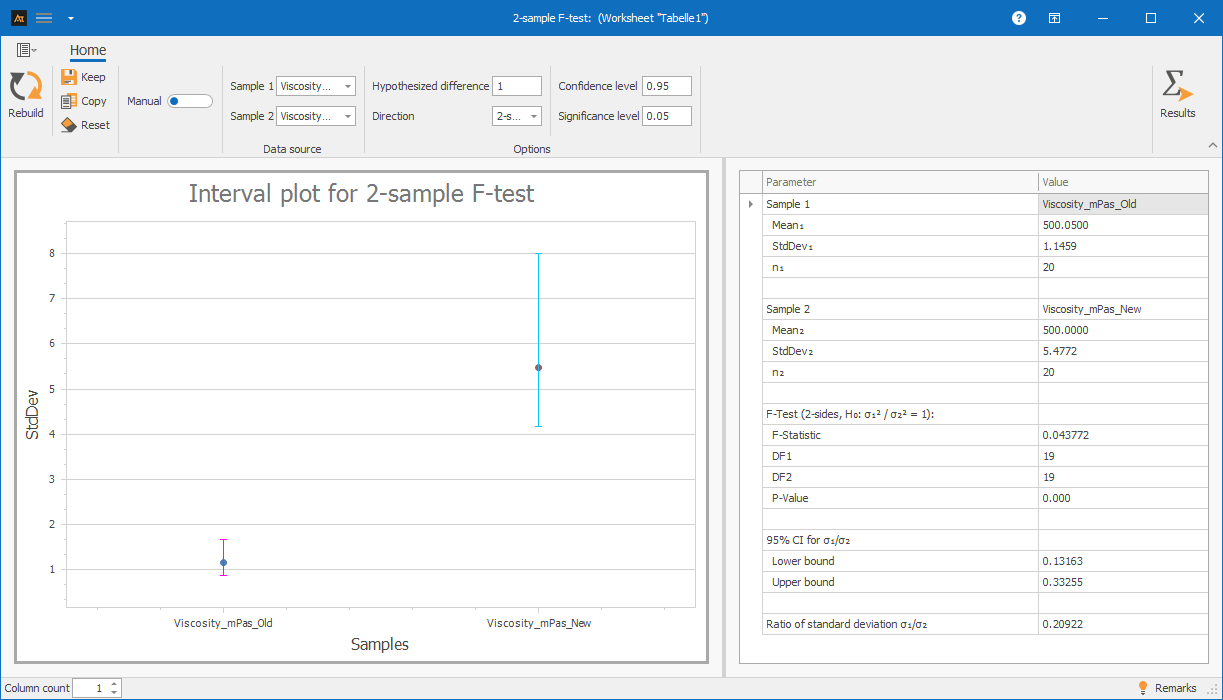
In product development, a new tomato sauce recipe is being tested. The goal is to determine whether the variation in viscosity of the new recipe differs from that of the previous recipe.
To this end, viscosity measurements are taken on samples of the old recipe and the new recipe. The measured values for both groups are collected independently of one another and treated as separate samples.
The F-test (two samples) will be used to determine whether the variances or standard deviations of the two groups differ statistically significantly.
Interpretation of the results:
The calculated p-value is well below the significance level of 0.05, so the null hypothesis is rejected. We conclude that the variability in viscosity between the old and new formulations is not the same. In this example, the new formulation shows significantly greater variability than the old one.
Explanations of the graph:
- The points mark the standard deviations of viscosity for the old and new formulations.
- The error bars represent the 95% confidence interval for the respective standard deviation.
- The non-overlapping confidence intervals also indicate that there is a difference in the standard deviation. The F-test confirms that this difference is statistically significant.
-
Procedure
(How was this graphic created?)
Preliminary Work
- Select a suitable measurement parameter whose variation is to be compared (e.g., viscosity).
- Define two groups whose variances or standard deviations are to be compared (e.g., viscosity of old vs. new formulation).
- Set the significance level (usually α = 0.05).
- Check whether the data show any signs of significant deviations from the normal distribution.
 Use in AlphadiTab
- In the Analyze phase, select the 2-Sample f-test tool.
- For Sample 1, enter “Viskositaet_mPas_Alt”.
- For Sample 2, enter “Viskositaet_mPas_Neu”.
- Perform the analysis by clicking “Create New.”
Interpretation
- Check whether the p-value is less than or equal to the significance level.
p ≤ α → statistically significant difference in variances or standard deviations.
p > α → no statistically significant difference in variances or standard deviations.Important: The interpretation refers exclusively to the standard deviation, not to the mean.
-
Adjustment options
Data
Manual entry:

The comparison is based on manually entered standard deviations and sample sizes for two samples.
Non-manual entry:

The comparison is based on the selected data columns.
Direction (hypothesis type)
The direction determines what type of difference between the two samples should be tested.
Double-sided
Null hypothesis
H₀: σ₁² / σ₂² = 1
Alternative hypothesis
H₁: σ₁² / σ₂² ≠ 1
Select “two-tailed” if you want to test whether the variances of the two samples differ, without specifying a particular direction.
- The test checks whether the variance of the first sample is greater or smaller than that of the second.
- This setting is useful when there is no specific expectation regarding the direction of the difference.
Example:
Do the variances in reaction times differ between Group A and Group B?
Larger
Null hypothesis
H₀: σ₁² / σ₂² = 1
Alternative hypothesis
H₁: σ₁² / σ₂² > 1
Select “Greater” if you want to check whether the variance of the first sample is greater than that of the second sample.
- The test only checks whether Sample 1 has significantly greater variation than Sample 2.
- Differences in the other direction are not taken into account.
Example:
Is the variation in delivery time greater before a measure is implemented than after?
Smaller
Null hypothesis
H₀: σ₁² / σ₂² ≥ 1
Alternative hypothesis
H₁: σ₁² / σ₂² < 1
Select “Smaller” if you want to check whether the variance of the first sample is smaller than that of the second sample.
- The test only checks whether Sample 1 has significantly lower variance than Sample 2.
- Differences in the opposite direction are not taken into account.
Example:
Is the variation in viscosity of the old formula smaller than that of the new one?
-
Requirements
Two groups
There must be exactly two groups whose variances or standard deviations are to be compared (e.g., old vs. new formula).
Why is this important?
The F-test is a method for comparing two variances.
Independent samples
The measured values of the two groups must not influence each other (no pairing of the same parts).
Why is this important?
The test assumes that the groups were collected independently of one another.
Continuous measurement data
The measured values should be continuous and sufficiently finely graded.
Why is this important?
The F-test compares variances of numerical measurement data.
Normally distributed data
The repeated measurement values should show no evidence of a significant deviation from the normal distribution.
Why is this important?
- The F-test relies heavily on the assumption of normally distributed data. In the event of significant deviations, the test results may be unreliable.
- In cases of highly skewed distributions or pronounced outliers, a robust variance test such as the Levene test should therefore be used instead.
-
Tools
(When are other options more suitable?)
If you need to compare the variances of more than two groups at the same time, robust methods such as the Levene test for multiple groups are more appropriate.
If the data is heavily skewed or contains significant outliers, a more robust method should be used.
If means are to be compared, a t-test or an ANOVA is more appropriate.
If proportions rather than variances are to be compared, a proportion test is the appropriate tool.
Production
Filling Volume of Tomato Sauce – Machine A vs. Machine B
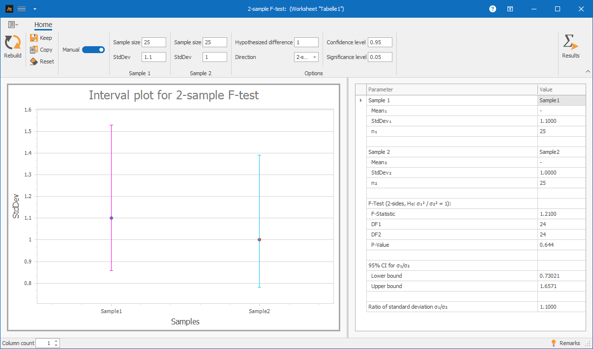
Two filling machines are used in production. The goal is to determine whether there is a difference in the variation of the fill volume between Machine A and Machine B.
Aggregated measurement data is available for both machines.
- Machine A: n = 25, mean = 500.2 ml, standard deviation = 1.1 ml
- Machine B: n = 25, mean = 498.9 ml, standard deviation = 1.0 ml
The variances are compared using an F-test (two samples).
Interpretation:
The F-test shows no statistically significant difference in the variance of the fill volume between the two machines. The p-value is 0.644, which is greater than 0.05, so the null hypothesis is retained.
IT help desks
Response time
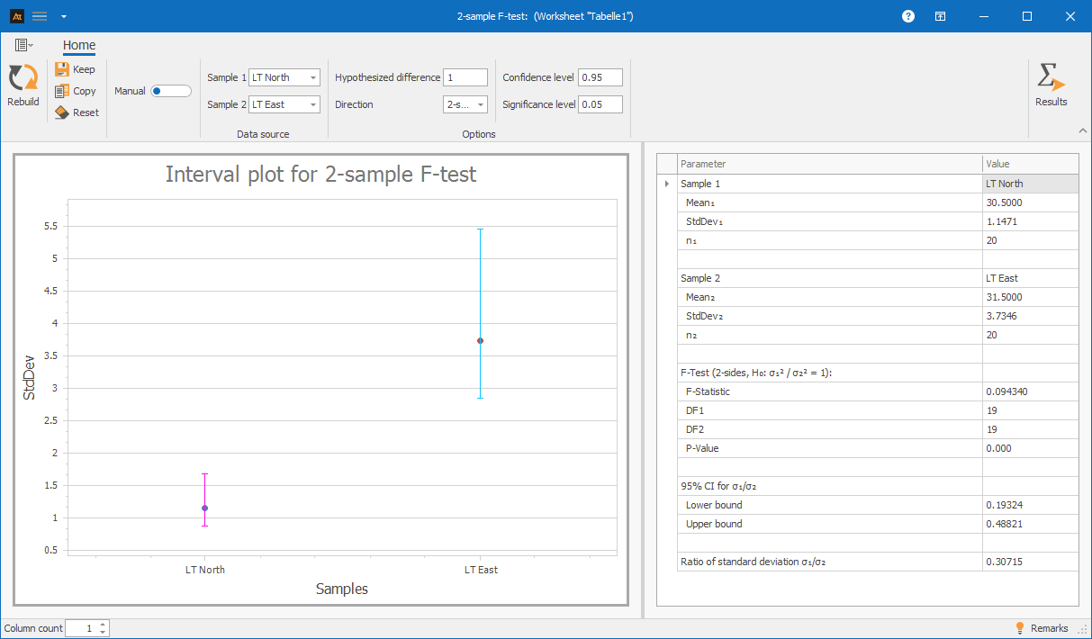
At the IT service desk, tickets are processed across multiple locations. Response times are regularly analyzed to identify variations in process stability.
In the example of IT tickets, data is available from three locations. The F-test (two-sample) is generally only suitable for comparing two groups.
If there are more than two locations, there are two possible approaches:
Pairwise comparisons using the F-test
Each location can be compared in pairs with the other locations (e.g., Location A vs. B, A vs. C, B vs. C). In each case, we check whether the variances in response times between two locations differ statistically significantly.
Alternative: Levene’s test across multiple groups
If all locations are to be considered simultaneously, a robust variance comparison across multiple groups is generally the more appropriate tool.
Note on interpretation
With multiple pairwise F-tests, the risk of chance hits increases. For an overall assessment of the locations, a procedure for multiple groups is therefore generally preferable.
Interpretation:
The F-test indicates a statistically significant difference between the variances in turnaround times at the DLZ North and DLZ East sites. The p-value is 0.000, which is below the significance level of 0.05.
From a statistical perspective, turnaround times at the East site vary significantly more than those at the North site.
Sales
Lead time by team
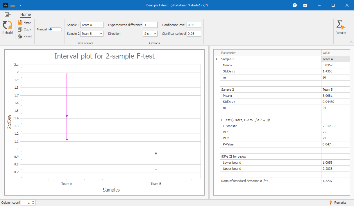
In the sales department, customer quotes are handled by two teams. The goal is to determine whether there is a difference in the variation of turnaround times between Team A and Team B.
Interpretation:
The F-test indicates a statistically significant difference in the variability of lead time between the two teams. The p-value is 0.047, which is just below 0.05, so the null hypothesis is rejected.
In this example, Team A exhibits greater variability in lead time and therefore operates less consistently than Team B.
Logistics
Delivery time to the logistics center
In the logistics department, customer orders are picked and shipped. New forklifts were introduced to increase efficiency.
The aim is to investigate whether the variation in delivery time (in hours) has decreased following the introduction of the new forklifts.
The analysis is performed using a two-sample F-test as a one-tailed test; in this case, “greater than” was selected.
H₀: σ_Before² / σ_After² ≤ 1
H₁: σ_Before² / σ_After² > 1
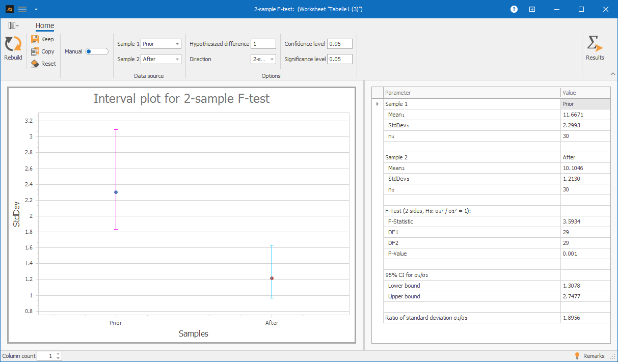
Interpretation:
The one-tailed F-test shows a statistically significant difference between the variances of delivery times before and after the introduction of the new forklifts (F = 3.5934; p = 0.000).
Since the p-value is below the significance level of 0.05, the null hypothesis is rejected. Delivery times before the introduction vary significantly more than after the introduction.
It can therefore be concluded that the introduction of the new forklifts not only affects the mean but, in this example, has also led to more stable delivery times.
Shopping
Supplier Comparison
The purchasing department sources components from two suppliers. The goal is to determine whether the variation in the scrap rate per shipment differs between Supplier A and Supplier B. The scrap rate is measured as a percentage for each shipment.
Note:
The F-test assumes that the metric data is approximately normally distributed.
Percentage values such as the scrap rate can be discrete, as they are derived from count data. With small delivery quantities, there are only a few possible percentage values. In such cases, the assumption of a normal distribution may be violated, and the F-test may not be appropriate.
For larger delivery quantities with many possible values, the F-test is generally acceptable in practice; if in doubt, a more robust method should be used.
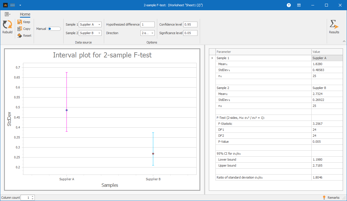
Interpretation:
The F-test indicates a statistically significant difference in the variance of the scrap rate among the suppliers (p = 0.005). The null hypothesis is rejected.
In this example, Supplier A exhibits the higher variance. Supplier B performs more consistently in terms of the scrap rate.
Planning
Forecast deviation
In production planning, demand forecasts are prepared for different planning periods. The forecast error is calculated to assess the quality of the forecast.
The aim is to investigate whether the variance of the forecast error differs between short-term and long-term planning periods.
Short-term planning horizon:
n = 30, standard deviation = 1.5%
Long-term planning horizon
n = 30, standard deviation = 3.8%
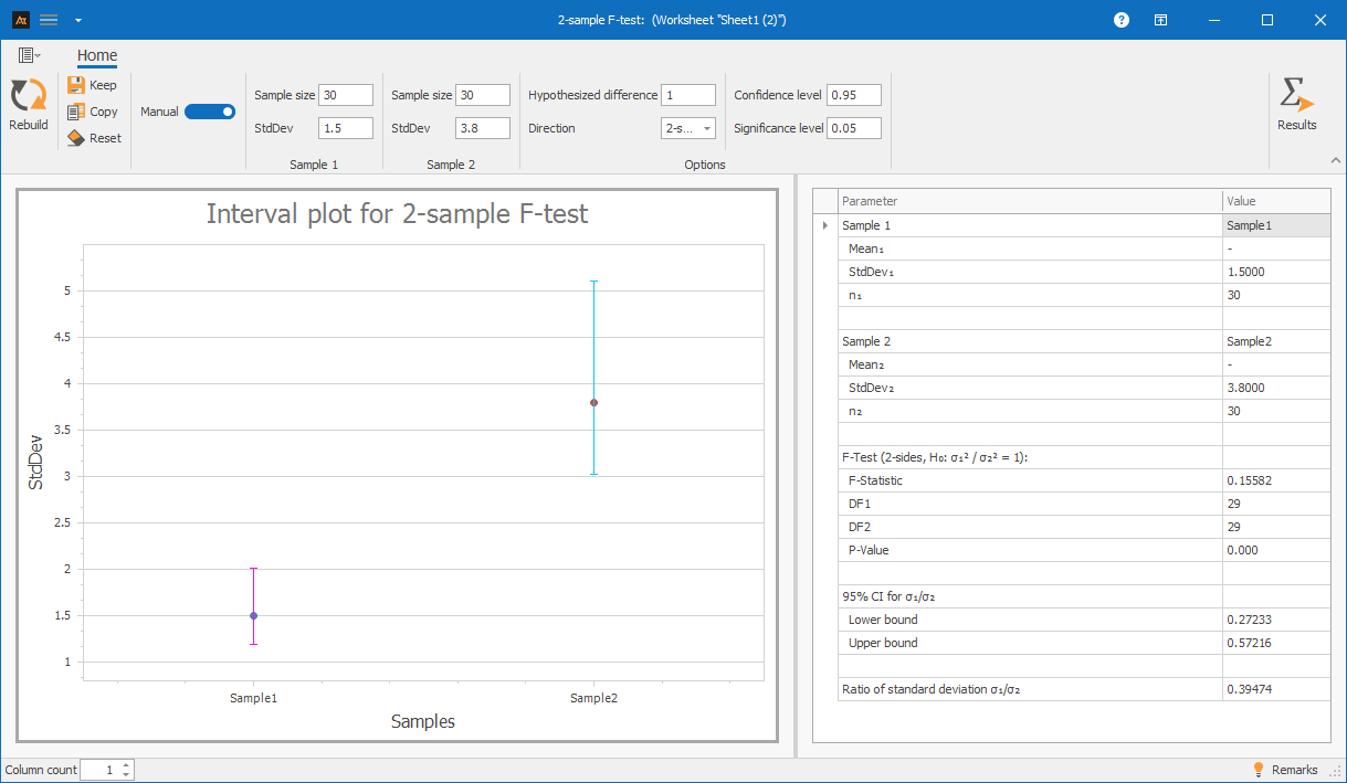
Interpretation:
The F-test for two independent samples shows that the variances of the short-term and long-term planning periods differ statistically significantly.
Since the p-value of 0.000 is below the significance level of 0.05, the null hypothesis is rejected.
There is thus statistical evidence that the forecast deviations vary much more widely in the long-term planning horizon than in the short-term one.
-
Terms
Continuous data: Data collected using a measuring instrument that may include both units and decimal places.
Normally distributed data: Data that can be well described by a normal distribution. This can be verified, for example, using a normality test.
x̄ = sample mean: The average value of the collected measurement data. It can be displayed in the output, but is not the actual test statistic of the F-test.
s = sample standard deviation: A measure of the dispersion of the data around the mean.
n = sample size: The number of observations within a sample.
α = Significance level: Specified probability of error with which the null hypothesis is incorrectly rejected.
p-value: Result of the hypothesis test used to make a decision between the two hypotheses.
F-value or F-statistic: Test statistic of the F-test. It is calculated from the ratio of the two sample variances.
DF1 / DF2 = Degrees of freedom: Values derived from the sample sizes of both groups that determine the shape of the F-distribution.
σ₁² / σ₂² = Variance ratio: Reference value of the test. Under the null hypothesis, this ratio is equal to 1.
Confidence level: Probability that the calculated confidence interval covers the true parameter value (e.g., 95%).
Confidence interval: Range of values that contains the true variance ratio at the chosen confidence level.
Null hypothesis: Initial hypothesis assuming equal variances or a variance ratio of 1. It is tested in the hypothesis test.
Alternative hypothesis: Counter-hypothesis to the null hypothesis. It describes the substantive research question, e.g., whether variances differ significantly.
Test direction: Indicates whether a difference is tested without specifying the direction (two-tailed) or with a specific direction (greater/lesser).
Two-tailed: Tests whether the variances differ, regardless of the direction.
Greater: Tests whether the variance of the first sample is greater than that of the second sample.
Smaller: Tests whether the variance of the first sample is smaller than that of the second sample.
Continuous data: Data collected using a measuring instrument that can have both units and decimal places.
Normally distributed data: Data that can be well described by a normal distribution. This can be verified, for example, using a normality test.
x̄ = Sample mean: The average value of the collected measurement data. It can be displayed in the output but is not the actual test statistic of the F-test.
s = Sample standard deviation: A measure of the dispersion of the data around the mean.
n = sample size: Number of observations within a sample.
α = significance level: Specified probability of error with which the null hypothesis is incorrectly rejected.
p-value: Result of the hypothesis test used to make a decision between the two hypotheses.
F-value or F-statistic: Test statistic of the F-test. It is calculated as the ratio of the two sample variances.
DF1 / DF2 = Degrees of freedom: Values derived from the sample sizes of both groups that determine the shape of the F-distribution.
σ₁² / σ₂² = Variance ratio: Reference value of the test. Under the null hypothesis, this ratio is equal to 1.
Confidence level: Probability that the calculated confidence interval covers the true parameter value (e.g., 95%).
Confidence interval: Range of values that contains the true variance ratio at the chosen confidence level.
Null hypothesis: Initial hypothesis assuming equal variances or a variance ratio of 1. It is tested in the hypothesis test.
Alternative hypothesis: The hypothesis that opposes the null hypothesis. It describes the substantive research question, e.g., whether variances differ significantly.
Test direction: Specifies whether a difference is tested without specifying the direction (two-tailed) or with a specific direction (greater/less).
Two-tailed: Tests whether the variances differ, regardless of the direction.
Greater: Tests whether the variance of the first sample is greater than that of the second sample.
Smaller: Tests whether the variance of the first sample is smaller than that of the second sample.
-
Formulas
F-test statistic
\( \mathrm{F}=\frac{\frac{\mathrm{s}_1^2}{\mathrm{s}_2^2}}{\mathrm{k}^2} \)
Degrees of freedom
\( \mathrm{df}_1=\mathrm{n}_1-1 \)
\( \mathrm{df}_2=\mathrm{n}_2-1 \)
Confidence interval (lower limit)
\( \mathrm{Lower\ Limit}=\sqrt{\frac{\mathrm{s}_1^2}{\mathrm{s}_2^2}\cdot \mathrm{F}_{\mathrm{low}}} \)
Confidence interval (upper limit)
\( \mathrm{Upper\ Limit}=\sqrt{\frac{\mathrm{s}_1^2}{\mathrm{s}_2^2}\cdot \mathrm{F}_{\mathrm{up}}} \)
Ratio of standard deviations
\( \frac{\mathrm{s}_1}{\mathrm{s}_2}=\sqrt{\frac{\mathrm{s}_1^2}{\mathrm{s}_2^2}} \)
Note: NMath was used to calculate the sample standard deviations as well as the distribution and quantile values of the F and chi-square distributions.
-
Keywords