Preliminary work
- Select a continuous measurement variable (e.g., viscosity).
- Select a suitable measuring device for determining the measured variable (e.g., rotational viscometer).
- Provide a reference part or reference sample (e.g., homogenized tomato sauce).
- Ensure that the specification limits are known (USG = 950, OSG = 1050).
- Define the measurement conditions and keep them constant during the measurement (same sample, same temperature, one tester; refer to the reference manual for the measuring instrument).
- Plan and perform a sufficient number of repeat measurements (e.g., 25 measurements).
 Use in AlphadiTab
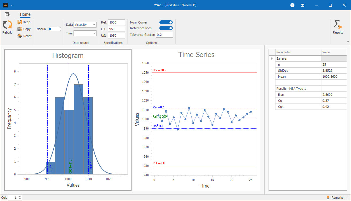
- In the Measure phase, call up the “MSA Type 1” function.
- Enter the “Viscosity” column for the data.
- Enter the reference value 1000 here, enter 950 for USG and 1050 for OSG.
- Click on the “Create new” button to perform MSA 1.
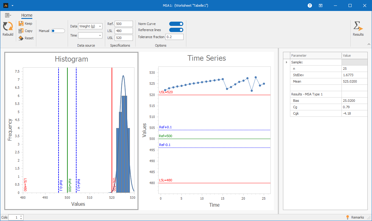
Interpretation
- First check whether the measuring device is capable (capable if the Cgk value is ≥ 1.33 or corresponds to the required minimum value).
- Then determine whether the position or dispersion of the measuring device (or both) needs improvement.
Continuous data
Continuous data is required to perform a type 1 measurement system analysis.
Why is this important?
Only with continuous data can the dispersion and position of the measuring instrument be evaluated. This data is collected exclusively with a measuring instrument and allows a quantitative assessment of the measurement capability.
Two specification limits
To calculate the Cg and Cgk key figures, both a lower and an upper specification or tolerance limit must be defined.
Why is this important?
Only with two specification limits can the dispersion of the measuring equipment be set in relation to the permissible tolerance range.
Reference part/reference sample
The analysis is based on repeated measurements of a single reference part or reference sample. This must remain stable throughout the entire measurement series and must not change.
Why is this important?
The aim of the analysis is to evaluate only the dispersion of the measuring instrument. If the reference sample is not stable, additional dispersion occurs that is not caused by the measuring instrument and distorts the result.
Constant measurement conditions
The sample, measuring equipment, tester, and environmental conditions (e.g., temperature) must be kept constant during the measurement.
Why is this important?
Only under constant conditions can it be ensured that observed fluctuations in the measured values are attributable exclusively to the measuring equipment.
Normally distributed data
The repeated measured values should not show any indications of a relevant deviation from the normal distribution, as the calculation of the Cg and Cgk key figures is based on assumptions of normal distribution.
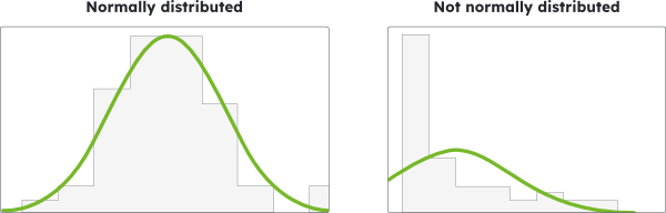
Why is this important?
If there is a significant deviation from the normal distribution, Cg and Cgk do not provide reliable information about the measurement capability.
This can make the evaluation of the measuring equipment dispersion inaccurate or misleading.