Purpose of the tool
Procedure
Settings
Interpretation guide
Forms of representation
Requirements
Tools
Examples
Terms
Formulas
Process Capability Analysis
-
Purpose of the tool
The purpose of process capability analysis is to evaluate the quality of processes by using the Cp and Cpk metrics to assess the location (accuracy) and dispersion (precision) of a characteristic. The higher the Cpk value, the better the process. A Cpk value of 1.33 or higher is often considered to indicate a capable process.
-
Example: Tomato Sauce
Viscosity plays a crucial role in the production of tomato sauce: if the sauce is too thin or too thick, it will not meet customer expectations. Cp and Cpk can be used to check whether the process reliably maintains the desired consistency.
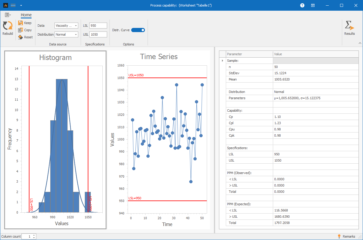
Interpretation of the results:
Here in the evaluation, you can see a Cp value of 1.10 and a Cpk value of 0.98. The Cpk value is lower than the frequently required reference value of 1.33 – the process is therefore not capable.
The Cp value of 1.10 shows that the dispersion of the process is still too high – the process is therefore not capable due to dispersion. Since Cpk is also slightly smaller than Cp, there is also a slight positional deviation. However, the main cause of the lack of process capability is clearly the excessive dispersion.
Explanations of the graph:
The bars represent the frequency distribution of the measured values.
The line is the normal distribution, which was created based on the mean and standard deviation of the actual data.
The narrower the curve, the better the process fits within the specification limits (USG and OSG).
-
Procedure
Below you will find the considerations and steps necessary to perform a process capability analysis.
Preliminary work
- Select a continuous measurement variable and collect measured values (e.g., viscosity).
- Check measured values for normal distribution
- Determine or request specification limits (e.g., USG = 950, OSG = 1050).
 Use in AlphadiTab
- In the Measure phase, select the Cp, Cpk tool
- Select “Viscosity” for data.
- Specify the specification limit: USG = 950, OSG = 1050
- Perform the analysis by clicking on the “New” button.
Interpretation
- First, check whether the process is capable (capable if the Cpk value is ≥ 1.33 or corresponds to the required minimum value).
- Then determine whether the location or the dispersion of the process (or both) needs improvement.
-
Requirements
Selecting the appropriate distribution for the data
To calculate Cp and Cpk, it is assumed that the data follows a distribution. Different formulas are stored for the various distributions, so the operator must select the appropriate distribution, for example, using the distribution test.
Why is this important?
Without the appropriate distribution, Cp and Cpk no longer correspond to the actual process performance.
This makes reject and risk assessments inaccurate or misleading.
Suitable measuring equipment
The data must be collected using reliable measuring equipment that is suitable for the characteristic in order to ensure correct results.
Why is this important?
If the measuring equipment is not capable, incorrect conclusions about the actual process performance may be drawn.
For example, it may appear that the process is not capable, even though the deviations are caused solely by the unsuitable measuring equipment.
-
Tools
(When are others more suitable?)
For nominal, ordinal, or discrete (countable) data, no process capability analysis with Cp and Cpk is performed, as these metrics require continuous, metric measurements.
-
Examples
Production
Filling quantity tomato sauce
In this example, the filling quantity of tomato sauce was examined. The filling quantity is measured using a suitable measuring device to check whether the machine reliably maintains the target quantity of 500 ml.
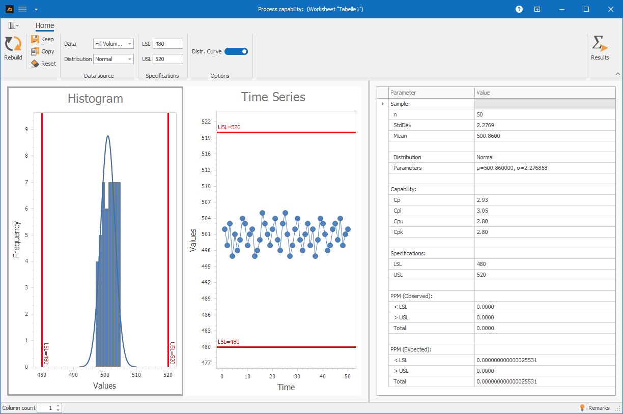
Interpretation
The evaluation yields a Cp value of 2.93 and a Cpk value of 2.80.
Both values are above the frequently required reference value of 1.33.
The process is capable.
The dispersion is small enough (Cp high).
The position is good (Cpk ≈ Cp).
Goods receipt/Logistics
Processing time for an order
In the goods receiving department, every order goes through an inspection step where delivery notes are checked and items are entered into the system. While some processes are handled quickly, others get stuck: a missing barcode, an incomplete delivery note, or a quick query can cause individual orders to be delayed. This results in very different processing times, which are clearly reflected in the measurement data.
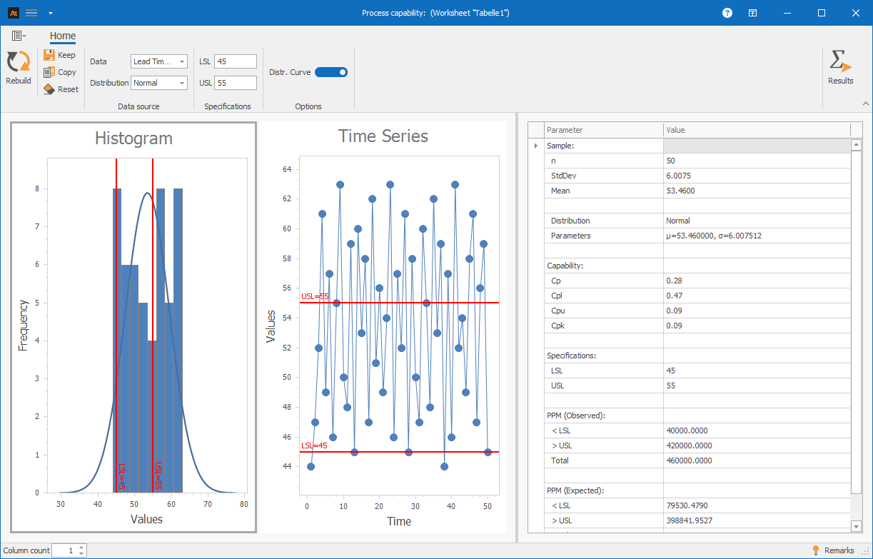
Calculated key figures
- Cp = 0.28
- Cpk = 0.09
Interpretation
The process is not capable.
- Cp < 1.33 → Dispersion too high, throughput times fluctuate greatly.
- Cpk < Cp → additional location problem (average is too close to a tolerance limit).
IT Support
Response time for inquiries
The IT service desk receives many different inquiries every day. Some tickets can be answered immediately because the solution is obvious or only a brief note is required. Other requests first require further inquiries, a system search, or the reproduction of an error. While simple cases are processed quickly, the response time for more complex tickets is significantly delayed. This results in very different response times—even though the goal is to keep the response time below 35 minutes.
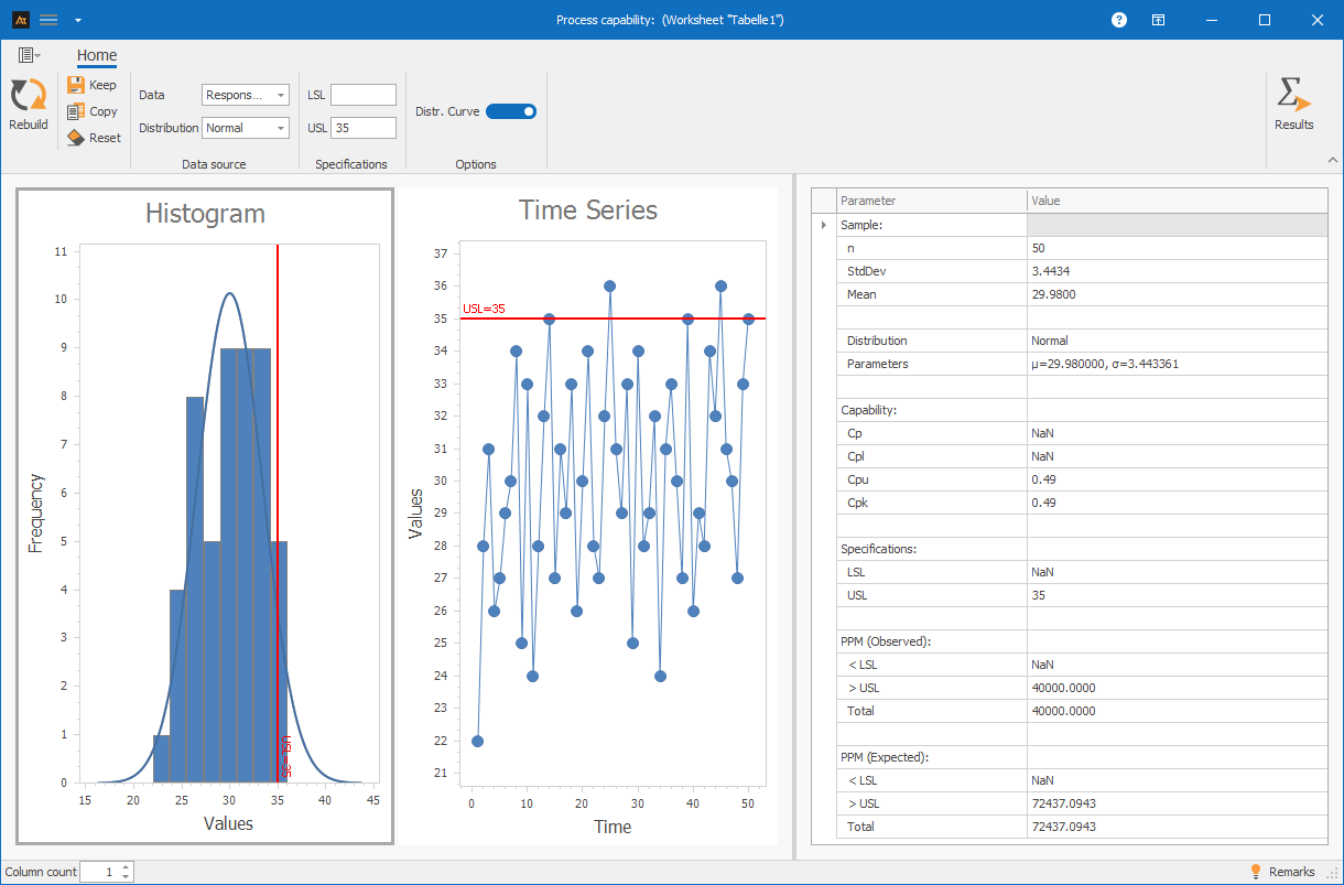
Calculated key figures
- Cp: cannot be calculated, as only one specification limit is available
- Cpk = 0.49
Interpretation
The process is not capable, as the Cpk value is significantly below the frequently required minimum value of 1.33.
Since only an upper specification limit is defined, the process can be optimized both by reducing the dispersion and by improving the location. Both would lead to a higher Cpk value and process capability.
-
Terms
Continuous data: Data that is recorded using a measuring device and can have both units and decimal places.
Normally distributed data: Data that can be well described by a normal distribution. This can be verified, for example, by testing for normal distribution.
OSG = OTG = Upper specification or tolerance limit: The maximum permissible value for the target variable. If a measured value is above this, it is considered unacceptable.
LSP = LTP = Lower specification or tolerance limit: The minimum permissible value for the target variable. If a measured value is below this, it is considered unacceptable.
Cp: Capability index that evaluates the dispersion of the process in relation to the specification limits.
Cpk: Capability index that evaluates both the dispersion and the position of the process in relation to the specification limits.
x̄ = Sample mean: Average value of the measured data collected.
s = Standard deviation of the sample: Measure of the dispersion of the data around the mean.
-
Formulas
Mean
\( \bar{\mathrm{x}}=\frac{1}{\mathrm{n}}\sum_{i=1}^{\mathrm{n}}\mathrm{x}_i \)
Standard deviation
\( \mathrm{s}=\sqrt{\frac{1}{\mathrm{n}-1}\sum_{i=1}^{\mathrm{n}}(\mathrm{x}_i-\bar{\mathrm{x}})^2} \)
Capability index Cp
\( \mathrm{C}_\mathrm{p}=\frac{\mathrm{OSG}-\mathrm{USG}}{6\,\mathrm{s}} \)
Capability index Cpk
\( \mathrm{C}_{\mathrm{pk}}=\min\!\left(\frac{\mathrm{OSG}-\bar{\mathrm{x}}}{3\,\mathrm{s}},\frac{\bar{\mathrm{x}}-\mathrm{USG}}{3\,\mathrm{s}}\right) \)
Notation:
x̄ = mean value of the sample
s = standard deviation of the sample
n = sample size
xi = i-th measured value
-
Keywords